Shallow Neural Networks for Trading: Why Simple Models Win
After 4 months of failed strategies, I tried machine learning. Here's what I learned.
The Story So Far
In my last post, I shared how testing momentum and mean reversion strategies for 4 months ended in a graveyard of deleted code. Cross-sectional momentum dropped 92% when tested on new data. Dual momentum offered 9% returns with a 53% drawdown. RSI mean reversion generated maybe 7 trades across an entire year. The strategies in books didn't work. So I tried something different.
Instead of rules-based systems with hardcoded thresholds, I explored models that could learn patterns from data. Not the deep learning architectures that dominate headlines - those require massive datasets and tend to overfit on financial time series. Something simpler. A neural network with a single hidden layer. A "shallow" MLP.
The results were surprising. Not because they were spectacular (this is finance, not ImageNet), but because they actually survived out-of-sample testing. They showed consistent performance across both stocks and cryptocurrency. This post explains how shallow MLPs work, why they're particularly suited for trading, and what I learned building one that actually performed.
What is a Multilayer Perceptron?
The multilayer perceptron (MLP) is one of the oldest neural network architectures, dating back to the 1980s. Despite being "old," it remains remarkably effective for many prediction tasks.
The architecture is straightforward:
graph LR
    subgraph Input["Input Layer<br/>(features)"]
        I1((SMA))
        I2((RSI))
        I3((Vol))
        I4((ROC))
        I5((...))
    end

    subgraph Hidden["Hidden Layer<br/>(learned)"]
        H1((H1))
        H2((H2))
        H3((H3))
        H4((H4))
    end

    subgraph Output["Output Layer<br/>(prediction)"]
        O1((Buy))
        O2((Hold))
        O3((Sell))
    end

    I1 --> H1 & H2 & H3 & H4
    I2 --> H1 & H2 & H3 & H4
    I3 --> H1 & H2 & H3 & H4
    I4 --> H1 & H2 & H3 & H4
    I5 --> H1 & H2 & H3 & H4

    H1 --> O1 & O2 & O3
    H2 --> O1 & O2 & O3
    H3 --> O1 & O2 & O3
    H4 --> O1 & O2 & O3
The input layer receives your features - whatever data you're feeding the model. For trading, this might be 30-50 engineered technical indicators. The hidden layer is where the "learning" happens. Each neuron takes a weighted sum of its inputs, transforms it through an activation function, and passes it forward. The weights are what the network learns during training. Finally, the output layer produces the prediction - for classification tasks, this might be probabilities for each class (Buy, Hold, Sell).
The key innovation that made MLPs trainable was the backpropagation algorithm, published by Rumelhart, Hinton, and Williams in their landmark 1986 Nature paper "Learning representations by back-propagating errors". Before this, training multi-layer networks was considered computationally infeasible.
The Activation Function: Why Non-Linearity Matters
Here's a mathematical fact that took researchers years to fully appreciate: if you stack multiple linear transformations, you get... one linear transformation. No matter how many layers you add, without non-linearity, your neural network can only learn linear relationships. This is where activation functions come in. They introduce non-linearity, allowing the network to learn complex patterns that linear models can't capture.
The Sigmoid (Logistic Function)
The sigmoid function was the original choice. Also known as the logistic function, it squashes any input to a value between 0 and 1:
This produces a smooth S-curve:
- Large negative inputs approach 0
- Zero input gives exactly 0.5
- Large positive inputs approach 1
The problem? When inputs are very large or very small, the function "saturates" - its output barely changes regardless of the input. During training, this causes gradients to nearly vanish, making learning painfully slow or impossible for deep networks. This is the infamous "vanishing gradient problem."
ReLU (Modern Default)
The Rectified Linear Unit (ReLU) is embarrassingly simple:
If the input is positive, pass it through unchanged. If negative, output zero. That's it.
| Input | Output |
|---|---|
| -5 | 0 |
| -1 | 0 |
| 0 | 0 |
| 3 | 3 |
| 10 | 10 |
No complex functions, no expensive exponential calculations. Yet this simple change revolutionized neural network training. Gradients flow cleanly through positive neurons, networks train faster, and the vanishing gradient problem largely disappears. For trading applications, ReLU's speed advantage matters. When you're retraining models daily or weekly on new data, training time adds up.
How the Network Learns: Backpropagation
Here is the updated section. Since you are specifically using a Sigmoid activation function, I have updated the math to show the specific derivative for it.
This is a great addition for CS students because the derivative of a Sigmoid function has a very clean, beautiful property: . This simplifies the implementation significantly and is a classic exam topic.
How the Network Learns: Backpropagation
Training a neural network is fundamentally about adjusting weights so the model's predictions match reality. The backpropagation algorithm makes this tractable, even for networks with millions of parameters.
The intuition is simple:
-
Forward Pass: Data flows through the network. Each neuron computes a weighted sum, applies the Sigmoid activation function, and passes the result forward.
-
Calculate Error: Compare the prediction to what actually happened. This error gets quantified by a Loss Function.
-
Backward Pass: Here's the clever part. The error signal flows backwards. At each connection, we calculate how much that specific weight contributed to the error.
-
Update Weights: Nudge each weight in the direction that would have reduced the error.
-
Repeat: Do this thousands of times until the weights converge.
-
The Mathematical Engine: The Chain Rule
For Computer Science students, "intuition" is only half the picture. The engine driving the Backward Pass is the Chain Rule of calculus.
We want to know how the total Loss changes if we wiggle a specific weight . Mathematically, we are looking for the gradient:
Because our network uses the Sigmoid function, defined as , we can be very precise about this.
If we look at a single neuron where and the output is , the Chain Rule breaks the derivative down into three terms:
Let's solve for the middle term, the derivative of the Sigmoid:
The derivative of the sigmoid function has a special property that makes it computationally efficient. It can be expressed using the output of the function itself:
So, substituting this back into our Chain Rule, the gradient for the weight becomes:
This equation is exactly what you would code in Python. It tells us that the update depends on the error, the current activation (how "active" the neuron is), and the input strength.
The Update Rule
Once we have this gradient, we perform the Gradient Descent update. We adjust the weight by subtracting the gradient multiplied by a learning rate :
An Analogy
Imagine learning to throw darts blindfolded. Someone tells you where each dart landed relative to the bullseye. "Too far left." "A bit high." After each throw, you adjust your technique slightly based on this feedback. Over hundreds of throws, you learn to hit the target consistently.
In this analogy, the "feedback" is the gradient (), and the "slight adjustment" is the learning rate (). Backpropagation is the mathematical machinery that automates this feedback loop.
Why "Shallow" Works for Financial Data
In 1989, George Cybenko proved the Universal Approximation Theorem: a neural network with just one hidden layer can approximate any continuous function to arbitrary precision, given enough neurons. Kurt Hornik and colleagues published similar results the same year.
This theorem is both liberating and misleading. Yes, a single hidden layer can theoretically learn anything. But "can" doesn't mean "should." The theorem says nothing about how many neurons you'd need, how long training would take, or how well the model would generalize to new data. For financial applications specifically, shallow networks have practical advantages over deep architectures:
Limited Data
Deep networks are data hungry. Computer vision models train on millions of images. Language models consume trillions of tokens. Financial time series? You might have a few thousand daily bars, and only a fraction of those represent the current market regime. With limited data, deep networks overfit. They memorize the training set instead of learning generalizable patterns. The 37% backtest return that becomes 3% out-of-sample - that's overfitting in action.
Shallow networks have fewer parameters, which constrains their capacity to memorize noise.
Regime Changes
Markets evolve. What worked in 2020 might fail in 2024. Strategies optimized for trending markets get destroyed in choppy conditions. Deep networks, with their millions of parameters tuned to historical patterns, struggle to adapt when regimes shift. Simpler models are more robust to distribution shift. They capture broader patterns rather than fine-grained historical quirks.
Regularization is Key
Even shallow networks can overfit. The solution is regularization - techniques that penalize model complexity and constrain what the network can learn.
Common approaches include:
- Weight penalties: Discourage large weights, forcing the network to find simpler solutions
- Early stopping: Stop training before the model memorizes the training data
- Dropout: Randomly disable neurons during training, preventing co-adaptation
In my testing, aggressive regularization made the difference between strategies that collapsed out-of-sample and ones that held up. The models that worked weren't just shallow - they were heavily constrained.
The Counterintuitive Finding
The network architecture that performed best was startlingly small. Not hundreds of neurons. Not even dozens. A handful of neurons in a single layer, with strong regularization, outperformed larger architectures. This isn't universally true, but it reflects something about financial prediction: the signal-to-noise ratio is terrible. Markets are efficient enough that any predictable patterns are subtle. More model capacity doesn't find more signal - it just memorizes more noise.
Feature Engineering: The Inputs That Matter
The features you feed your model matter at least as much as the model architecture. "Shit in, shit out" (or SiSo for short) applies relentlessly. For trading, features typically derive from price action, momentum indicators, volatility measures, and volume. The specific combination matters less than two critical practices:
Lag-shifting: Every feature must be lag-shifted by at least one period. If your feature uses today's close to predict today's direction, you've leaked future information. The model will look amazing in backtests and fail completely in production. This "look-ahead bias" is the most common mistake in trading system development.
Feature scaling: MLPs are sensitive to input scale. Before training, features should be normalized to consistent ranges.
What We're Predicting
The model needs a target - what are we actually trying to predict? For trading, the most direct target is future returns over some horizon. "Will the price be higher or lower in N days?" This can be framed as:
Classification: Predict discrete categories (Buy/Sell/Hold) based on whether returns exceed some threshold.
Regression: Predict the actual return value and convert to signals based on the prediction magnitude.
Both approaches work. Classification is more common because it directly maps to trading decisions.
Results: What I Found
After building out the infrastructure - feature engineering, model training, and walk-forward validation - I ran the shallow MLP against the same evaluation pipeline that crushed my momentum and mean reversion strategies.
Walk-Forward Validation: Train on historical data, test on the next period, roll forward, repeat. This simulates what would have happened if you'd actually traded the strategy, retraining as new data arrived. No peeking at future data, no optimizing on the test set.
The Contrast with Failed Strategies
The strategies from my previous post all failed out-of-sample validation. Here's the same-asset comparison:
META:
| Strategy | In-Sample | Out-of-Sample | Sharpe (OOS) | Max DD (OOS) | Trades (OOS) |
|---|---|---|---|---|---|
| RSI Mean Reversion | +150% | -60% | 0.04 | -99.9% | 167 |
| Shallow MLP | +40% | +115% | 2.09 | -39% | 46 |
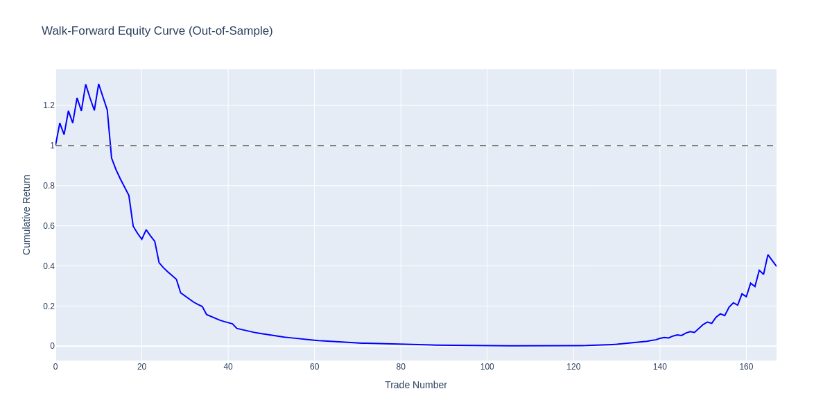 RSI Mean Reversion walk-forward equity curve: The strategy briefly peaked at ~1.3x around trade 10, then collapsed to near zero before a late partial recovery. Final value: 0.45x (-55% from start).
 Per-window returns for RSI: Windows 5-28 were almost entirely red (losses), with the model only finding success in later windows (30-50) that captured a different market regime.
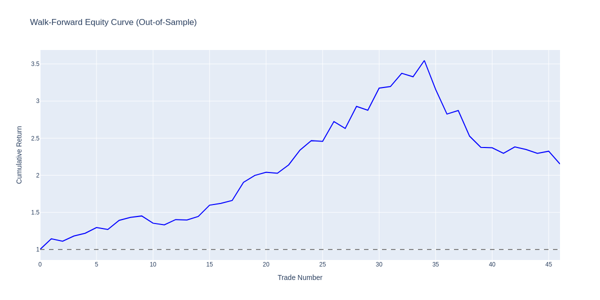
Walk-forward equity curve: Out-of-sample cumulative returns across 46 trades. The strategy peaked at ~3.5x before experiencing a drawdown, ending at ~2.15x (115% total return).
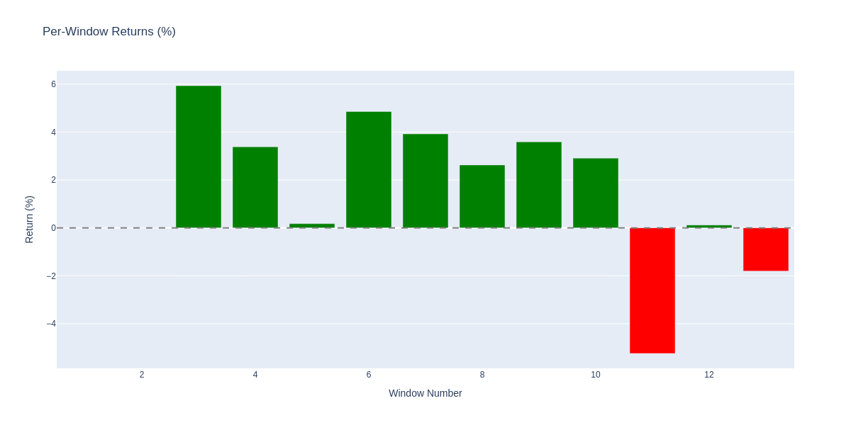 Per-window returns: Green bars show profitable walk-forward windows, red bars show losses. Most windows were profitable, with losses concentrated in later periods.
RSI mean reversion looked amazing in backtesting: +150% returns. But when subjected to the same walk-forward validation as the MLP, it doesn't just underperform - it loses 60% of capital with a near-total 99.9% max drawdown. The strategy got crushed during META's 2022 crash, triggering stop-losses repeatedly while attempting to "buy the dip" on a stock in freefall.
This is why out-of-sample testing matters. The 150% backtest return was an illusion - curve-fitted to historical data that couldn't predict future regimes.
The trade counts also matter. RSI mean reversion generated 167 trades because it kept triggering buy signals during the crash, only to hit stop-losses repeatedly. MLP's 46 trades were more selective and survived the drawdown with a manageable -39% max DD versus RSI's catastrophic -99.9%.
The MLP didn't show the catastrophic out-of-sample degradation that plagued the rules-based strategies. The regularization and simplicity paid off.
This isn't a guarantee of future performance - nothing is - but it cleared the validation hurdles that had filtered out everything else I'd tested.
Advantages and Disadvantages
No model is universally superior. Here's my take on the pros and cons of shallow MLPs for trading:
| Advantages | Disadvantages |
|---|---|
| Captures non-linear relationships that linear models miss | Requires feature engineering and domain knowledge |
| Fast training - seconds on a laptop, enables frequent retraining | Sensitive to input scaling - normalization is mandatory |
| Produces probability estimates for position sizing | Overfitting risk without proper regularization |
| Flexible inputs - any technical indicator works | Needs sufficient training data - rare signals don't work |
| More interpretable than deep learning architectures | Still less transparent than rule-based systems |
Conclusion
The strategies in books didn't work. What actually worked was simpler than I expected and a nostalgic walk through my 2nd year of university: a shallow neural network with a single hidden layer, aggressive regularization, and basic technical indicators as features.
The key insight isn't that MLPs are magic. It's that in domains with limited data and changing regimes - like financial markets - simple models that handle overfitting often beat complex ones. More parameters don't mean more predictive power. Sometimes they just mean more opportunities to fit noise.
If you're building trading systems, my recommendations:
-
Test obsessively. Backtest results without out-of-sample validation are meaningless. Use walk-forward testing. Never trust a strategy until it performs on data it's never seen.
-
Start simple. A tiny network with strong regularization is a better starting point than a deep architecture. Add complexity only if simple approaches fail.
-
Regularize aggressively. Weight penalties, early stopping, validation splits. Use every tool available to prevent overfitting.
-
Lag-shift everything. Look-ahead bias will make any strategy look good in backtests. Check your feature timing obsessively.
-
Expect modest results. Finance isn't computer vision. The signal-to-noise ratio is terrible. A Sharpe above 1.5 is excellent. Strategies claiming 10x returns should be viewed with extreme skepticism.
I'm still searching for what works. The shallow MLP is the first approach that cleared my validation hurdles. That's not proof it will work in the future - it's just the starting point for live testing.
The difference between this and my momentum journey? This one passed the tests before I traded it with real money. That's progress.
References
-
Rumelhart, D. E., Hinton, G. E., & Williams, R. J. (1986). Learning representations by back-propagating errors. Nature, 323(6088), 533-536. Link
-
Cybenko, G. (1989). Approximation by superpositions of a sigmoidal function. Mathematics of Control, Signals and Systems, 2(4), 303-314.
-
Hornik, K., Stinchcombe, M., & White, H. (1989). Multilayer feedforward networks are universal approximators. Neural Networks, 2(5), 359-366. Link
-
Namdari, A., & Durrani, T. S. (2021). A Multilayer Feedforward Perceptron Model in Neural Networks for Predicting Stock Market Short-term Trends. SN Operations Research Forum, 2, 71. Link
Previous post: Why Basic Momentum and Mean Reversion Don't Work Anymore